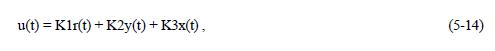
The controller algorithms are described in the following with these signals used in the formulas:
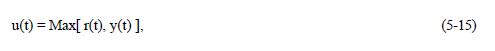
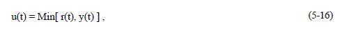
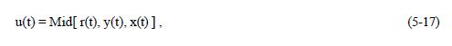
r(t) - Setpoint
y(t) - Measured Variable
u(t) - Output
x(t) - Output Tracking Variable
e(t) - Error between Setpoint and Measured Variable
T - Sample Interval
1. ANN
The detailed algorithm for the 1-For-3 ANN controller is lengthy and patented. We will just give a conceptual formula in the following:
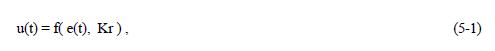
where Kr is the ANN Response Knob. The ANN weighting factors are updating at every sample through some learning algorithms and need not to be tuned manually.
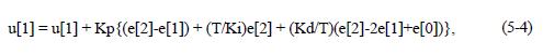
2. PID Standard

where e(t) = r(t) - y(t); This formula is the analog version in time domain. The digital version of the PID is as follows:

where e[0], e[1], and e[2] are the time sampled error signal e(t), e[2] is the current sample of e(t), and u[1] is the current sample of u(t). Kp is the Proportional Gain, Ki is the Integral Gain in second/repeat, and Kd is the Derivative Gain in repeat/second.
3. PID Error-Squared
and,
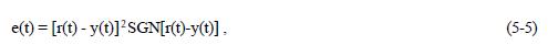
where SGN is the sign function.
4. PID Error-Squared
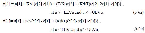
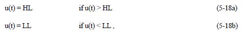
where LLVu is the Lower Limit Value of u, and
ULVu is the Upper Limit Value of u.
Notice that the controller output is always in range of 0 to 100 percent no matter what the LLVu and ULVu are.
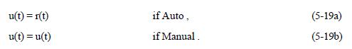
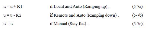
5. Ramp
6. Integrator
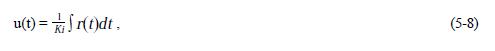
where r(t) is the input. The formula is an analog version, and its digital version is as follows:
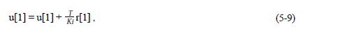
where, u[1] and r[1] are the current samples of u(t) and r(t), respectively.
7. Lead-Lag
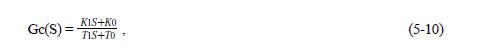
where Gc(S) = U(S)/R(S), which is the Laplace transfer function of the lead-lag block.
8. Second-Order Filter
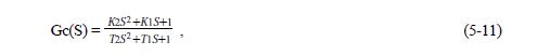
where Gc(S) is the Laplace transfer function of the block.
9. Dead-time
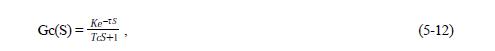
where Gc(S) is the Laplace transfer function of the block, K is the DC gain, Tc is the time constant, and t (Tau) is the dead time.
10. Linear
11. Ratio
12. High Select
13. Low Select
14. Middle Select
15. Limit
16. Loader