PID Control
The Proportional-Integral-Derivative (PID) is still the most popular controller used in industry today. We assume the user of this product is familiar with PID already so the details of the PID will not be discussed here. There are a few issues we would like to emphasize regarding the PID controller:
Different PID Types
There are many PID algorithms used in industry due to the pneumatic- to-analog and analog-to-digital evolution that PID took place. Basically, there are three major PID controller types that most PID algorithms could fit into. They are:
1) Noninteracting:

2) Parallel:

3) Interacting:

where Kp, Ki, and Kd can be called with different names, denoted with different symbols, and used with different units. All of these adds more headache and confusion to the PID users.
Tuning of PID
As discussed in Chapter 1, PID must be tuned properly to do its job. There are many books talking about different tuning methods. However, the principles are quite similar.
Firstly you need to know the approximate model of the process with DC Gain K, Time Constant Tc, and Dead Time Tau. Then you can use some formulas to calculate Kp, Ki, and Kd based on K, Tc, and Tau. The most famous formula is the one proposed by Zieglar and Nichols in 1942, which is still used by many people today. Later versions have improved this formula one way or the other based on some optimal criteria. These formulas work well if the model is accurate enough and the dynamics of the process do not change after the PID is tuned properly [21]-[25].
Self-Tuning of PID
For those processes whose dynamics change frequently, the PID controller needs to be tuned again and again to compensate for the changes. This creates a lot of trouble in real applications. In this case, self-tuning of PID is desirable. Self-tuning means that the PID tuning parameters can be updated automatically by itself without operator's attention. Basically, there are two ways to do it:
1) Model Based PID Self-Tuning
The process model is obtained online with some adaptive modeling techniques and then the PID parameters are updated based on the model. The ONSPEC PID Self-Tuner is one example of this type of product available on the market [28][33].
2) Rule Based PID Self-Tuning
The PID parameters are calculated and updated based on a set of pre-defined rules and some online data. [28]
PID Should be Replaced by the 1-For-3 ANN
In Chapter 1 and Chapter 2, we have spent much time talking about the reasons why PID should be replaced and how ANN is going to replace PID. If you have not read these chapters, it may be the time for you to visit them.
Cascade Control
Cascade control is one of the most useful schemes in process control. The key points of cascade control are as follows:
- A process has two or more major potential disturbances.
- The process can be divided into two loops, one is fast and one is slow.
- Use cascade control to take corrective action on disturbances more promptly.
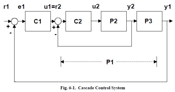
As shown in Figure 6-1, there are two controllers, the primary controller (C1) and the secondary controller (C2). The output of C1 drives the setpoint of C2.
Actually, process 1 combines the process and C2.
The problems of cascade control include:
- If PI or PID are used in cascade control, we need to tune 4 or 6 parameters properly.
- The interconnection of the primary loop and the secondary loop could cause system stability problems.
- If the process dynamics change frequently, the control performance is difficult to maintain.
When the 1-For-3 ANN controllers are used in a cascade control system, the tuning problems would be much easier to resolve since the ANN controller basically does not need tuning or can be tuned easily since you deal with only one tuning parameter for each loop.
How to Set Up a Cascade Control Loop
Let C1 be the primary controller and C2 be the secondary controller. The rules and steps to set up the cascade control loop are as follows:
1) Make sure C2 deals with the faster inner loop and C1 deals with the slower outer loop. That is, Tc2 < Tc1, and therefore, the sample interval selected would be T2 < T1.
2) The tuning and setup of the controllers in a cascade control system shall be carried out from the inside out; that is, the inner loop must be tuned and working first, then the outer loop can be closed and tuned. It can be seen that the inner loop is part of the process for the outer loop. Therefore, run the inner loop and tune the C2 as usual.
3) The inner loop is not difficult to work with since it is really just a single loop system. You should always make the inner loop run and tune it properly before attempting to close the outer loop.
4) Once C2 is doing its job properly, set the Remote/Local switch of C2 to Remote. This means that you request a remote setpoint from C1.
5) It is desirable to make a smooth transition to close the outer loop. Remember you have assigned C2 as the Secondary Controller while you were configuring C1 (Refer to the topic of Control Block and Faceplate Menu). Now, C1 is supposed to be in Manual, and OP1 is tracking MV2 as a standard feature implemented in the controller. That is,
OP1 -> MV2, when C1 is in Manual, and C2 is in Local
6) When C1 is in Manual, it will keep looking for that Remote/Local signal from C2. Once C1 sees a Local to Remote switch from C2, it will force its output track the setpoint of C2 immediately. That is,
OP1 -> SP2. when C1 is in Manual, C2 is in Remote.
7) C1 checks if there is no error and OP1 -> SP2, it will switch to Auto and force S2 -> OP1. The loops then are cascaded.
8) Tune the outer loop. Be careful not to tune C2 and C1 at the same time since once the tuning of C2 is changed, the process dynamics for process 1 are also changed.
Smith Predictor Dead-Time Control
As shown in Fig. 6-2, a Smith Predictor G2(S) is an internal model of the process G1(S) that can compensate the dead time, where
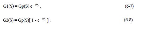
The reason why it works can be seen from the following analysis of the closed-loop transfer function of the system.
If the system is without a Smith Predictor, the dead-time is a major factor to its dynamics:
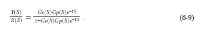
where Y(S)/R(S) is the closed-loop transfer function of the system.
The system with a Smith Predictor, the dead-time is canceled out:
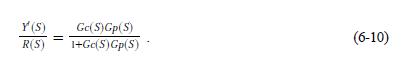
The Smith Predictor works in a quite ideal situation since it requires a precise process model. Also, if the process dynamics and dead time vary, the control performance will be difficult to maintain. However, if a 1-For-3 ANN controller is used together with a Smith Predictor for the process with large Tau-T Ratios, the control performance can be improved.
Feedforward Control
If a process has a significant potential disturbance which can be measured, we could use a feedforward controller to compensate the disturbance before the feedback loop takes corrective action. If the disturbance cannot be measured, feedforward control cannot be applied. If a feedforward controller is used properly together with a feedback controller, it can improve the control system greatly with small investment.
A Feedforward-Feedback control system is illustrated in Figure 6-3. Notice that, when the outputs of the feedback and feedforward controllers are summed, the presence of the feedforward controller affects the loop response to the disturbance only. That is, it does not affect the loop response to the setpoint. This is called the Invariant Principal.
Since the control objective for the feedforward controller is to compensate the measured disturbance, that is, we want
where Gf(S) is the Laplace transfer function of the feedforward loop. Based on this equation, the feedforward controller can be designed as

where Gfc(S) is the Laplace transfer function of the feedforward controller.
Feedforward compensation can be a simple ratio between two signals or some complex material and energy balance calculations involving the measured disturbances and the manipulated variable. If the process model, namely G1(S) and G2(S) cannot be found accurately, we could still use a simple dynamic block such as a lead-lag block to do the feedforward compensation since the disturbance remaining can be compensated by the feedback controller. With an ANN as the feedback controller and a lead-lag block as the feedforward controller, the whole system should work very well with minimum design and tuning efforts.
Ratio Control
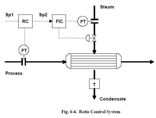
Ratio control is the simplest form of feedforward control. If a process mixes two or more streams together continuously to maintain a steady composition in the resulting mixture, or the establishment of a ratio between two flows is required, Ratio Control could be used.
Fig. 6-4 shows an example of ratio control between the steam and process inflows of a steam heater. Here the inflow is the disturbance or "wild" flow, and the steam is the manipulated flow. The steam flow is controlled by the FT with a setpoint that is a ratio of the inflow. This way, the outflow temperature is kept constant as long as the steam latent heat and inflow temperature remain constant. If the inflow could change wildly and the ratio control is not used, it would be very difficult to maintain the outflow temperature. Ratio control is quite useful and easy to implement.
Setpoint Control or Supervisory Control
In process control applications, the main control objective is usually to make the measured variable (MV) track the setpoint (SP). Once the loop is in automatic control and tuned properly, this control objective should be reached.
In many applications, what we try to achieve from a system engineering point of view is to increase productivity, efficiency, and product quality. To achieve these goals, optimization techniques need to be used.
Optimization means that we try to make the system run in some optimal states based on some criteria. Frequently, the solution of an optimization problem is based on a time or event related trajectory a variable should follow. For instance, the temperature of a chemical reactor should follow a trajectory to archive maximum productivity. To make the setpoint track a trajectory for optimization purposes is sometimes called Setpoint Control. It is also called Supervisory Control since it provides supervision for the control system.
The task to find optimal trajectories is related to each application. However, once the trajectory is determined, how to use it is what we will discuss here. There are several control blocks implemented in this product for Setpoint Control:
Ramping Block:
In many batch control applications, certain variables in a system need to be changed based on a schedule or some events. For instance, the temperature of a reactor should be raised up gradually, maintained for a certain period of time, and then brought down gradually. A Ramping block can be used to make this kind of setpoint trajectory. You can select the sample interval T and the Ramping Up and Ramping Down in the Configurator to form the trajectory.
Loader Block
A Loader Block is simply a fancy switch that is implemented in a faceplate fashion. If it is in Manual, its output can be selected. If it is in Auto, its output is forced to be equal to its setpoint which should be tied to a trajectory.
Steps For Setpoint Control
1) Assume you have determined the optimal trajectory for the reactor temperature.
2) The trajectory is often represented as a set of functions or a function with a set of conditions and constraints. Convert and implement this function by using the ONSPEC Command Language (OCL). If the function is simple, you may just need a linear or ramping block.
3) Connect all the variables properly by using the Configurator. It is recommended that a loader block be used to monitor and manipulate the Setpoint Control switch if you are not using a calculation block such as the ramping block.