Process Stability Requirement
The process to be controlled must be open-loop stable. That is, for any bounded process input, the process output is also bounded. This is called bounded-input-bounded-output (BIBO) stable. To test the behavior of your process, leave the loop in Manual, set the valve position (or the OP variable) to a certain value, and see if the measured variable is bounded.
If the process is not open-loop stable, it can be stabilized, for instance, by adding a feedback loop with a gain to the process. Then the stabilized system is treated as the process to be controlled. [55].
According to the stability criteria developed in the Model-Free Adaptive Control Theory, the 1 For 3 ANN controller may be able to control open-loop unstable processes such as the pH loop, it is still highly recommended that the user stabilize the loop before applying the ANN controller.
System Hardware Requirement
As a common practice, you need to select the proper size and types of control valves and sensors. Test and calibrate the equipment properly after the installation. Analysis has shown that about 80 percent of control system troubles are caused by hardware failures. Therefore, pay good attention to these issues before working with the controllers.
Process Approximation Model
Most of the open-loop stable process in industry can be approximated by a simple first-order-plus-delay model with the following Laplace transfer function:
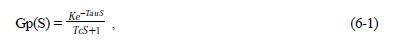
where, K - DC Gain, Tc - Time Constant, Tau - Dead Time.
DC Gain is the steady-state process output over the steady-state process input. Notice that the name DC Gain is based on the fact that, in steady state, f ->0, as t -> º. f->0 implies that the signal is DC signal (not AC signal).
Time Constant is the transition time it takes for the process output to reach about 68 percent of its steady-state value due to a step change of the process input. Notice that it is the constant that determines the first order lag of the step response. Most dynamic systems have a time constant no matter how quickly its output may respond to the input, since an output always needs some transition time to reach its steady state.
Dead Time is the pure time it takes for the process output to respond to the change of process input.
We could just consider these three parameters as qualitative information of the process to help setting up the ANN controller. You may not need to do serious experiments to determine these model parameters. All you have to do is to guess these parameters by your experience. Of course, you can do an open-loop or closed-loop bump test to make your guess easier. See References [21][25] for more information about the process models and the ways to find them..
DC Gain K
As a common practice, you need to scale the process input and output signals properly to make the process DC gain K -> 1. This will allow the valves and sensors to work in their full range.
Example: If MV is changing between 100 to 500, re-scale it through the conversion function in the ONSPEC I/O template to make it change between 0 to 100. Then K=(100-0)/(100-0)=1.
Nominal DC Gain
For a nonlinear process, the DC Gain may change in different ranges. It is desirable to set the Nominal DC Gain -> 1. A nominal value is usually defined as the value in the normal situation. Nominal DC Gain should be selected with a value in the middle of the uncertainty range.
Example: if 1 < K < 5, then Nominal DC Gain = 3. It is better to scale the signal to make 1/3 < K < 5/3. Then the Nominal DC Gain = 1.
Normalized DC Gain Kn
In case the engineering units need to be used in the system, the ULV and LLV need to be set properly according to the engineering unit. The ANN controller is designed to work with this situation by normalizing the input signals to the controller. In this way, a variable called the Normalized DC Gain Kn is used in the controller.
Example: SP and MV change in the range of 590 to 610, and OP changes in the range of 0 to 100. K = (610-590)/(100-0) = 20/100 = 0.2. However, if you specify the ULV= 610 and LLV=590, the controller will convert 590-610 to 0-100 through a normalization calculation. Then, the normalized DC Gain Kn = (100-0)/(100-0) = 1. Notice that if ULV=100 and LLV=0, K=Kn.
Limitations of the DC Gain
Since the ANN controller is implemented in digital version, the Sample Interval should be selected properly like the other digital control algorithms.
The rule of thumb for setting the T is as follows:
Sample Interval T = (Dominant Time Constant Tc)/20 ,
(6-2)
However, you do not need to find the precise time constant. As long as the time constant Tc is between 10T and 30T, no special adjustment is necessary.
For time-variant process where Tc changes through time, T should be calculated based on the Nominal Tc which again is the middle value within its uncertainty range.
Example: We guess that Tc changes between 100 and 200, then Nominal Tc = (200-100)/2 = 150. T = 150/20 = 7.5. Round the value off to get T=8. If you have a batch process that Tc changes in a very large scale, T has to be set accordingly. In ONPanel, you can change T automatically with Panel Code.
Dead-Time Tau
It is usually not meaningful to talk about the absolute value of the dead time since how the dead time affects the process dynamics is related to the time constant. We often use Tau-T Ratio as an important figure to measure the effect of the dead time. Tau-T Ratio is defined as:
Tau-T Ratio = Dead-time/Time Constant = Tau/T.
(6-3)
We know that a PID controller will work if Tau-T Ratio <= 2. Experiments show that ANN controller could work under a looser condition: Tau-T Ratio <= 4. That is if the dead time Tau < 4Tc, no special adjustment is needed. For most processes, this condition is satisfied. In case Tau-T Ratio is bigger than 4, a special treatment needs to be considered. For instance, you can use a Smith Predictor as an internal model to compensate the effect of the dead time. See the topic of Smith Predictor Dead Time Control for more details.
ANN Response Knob Kr
In practice, we do not need to do experiments in order to use the ANN controller. This is a major advantage of ANN control compared to PID and other advanced control techniques. If we have some knowledge about the K, Tc and the Tau-T Ratio, we will be OK.
Nevertheless, a tuning parameter called the ANN Response Knob Kr is left in the design so that you can shape up the loop as you wish. For instance, if you want the closed-loop step response to have less or no overshoot, just tune the Kr smaller. If the conditions of K, Tc, and Tau mentioned previously are satisfied, you can just leave the ANN Response Knob Kr=50. The system should work fine.
The range of Kr: 0 to 100 percent. Default value: 50 percent.
Bumpless Transfer of the ANN Controller
It is desirable to have a smooth transition to close a control loop in applications. That is, when the controller is switched from Manual to Auto, we do not want the controller output u(t) to upset the valve position OP. This is called bumpless transfer. The steps to make a bumpless transfer are as follows:
1) Assume that you have a new loop, the controller is in Manual and you have configured the controller properly. Now, set the valve position OP to a nominal value, for instance 50 percent.
2) The measured variable MV starts to track OP. It generates the so called open-loop step response.
3) Wait until MV is about steady, that is, MV stops changing or changes very slowly.
4) If you are using the faceplate instrument in ONSPEC, press the Setpoint Tracking button to turn it from OFF to ON. It will make SP track MV for just one time cycle. The Auto/Manual button will be disabled when ST flag is ON because the controller needs several cycles to adjust itself to make controller output u(t) track the valve position OP.
5) A few time intervals later, the ST flag will be reset by the controller and you can press the Auto/Manual switch to close the loop. Then, OP will be forced to equal to u(t). If OP -> u(t) before the switch from Manual to Auto, there should have no bump to make OP have wild changes.
Clever Use of the 1-For-3 ANN Controller
Although the 1-For-3 Controller is as powerful as we have described, it is still a single-input-single-output controller for analog signals. To apply it in your applications successfully, you may need to incorporate it with some established control schemes and strategies.
For example, a process that requires a PID controller and a feedforward ratio block should be designed with an ANN and a ratio block.
As a complete control product, the 1-For-3 Control Pack includes 15 most popular control algorithms. The following section will review and highlight some control schemes such as the cascade control and feedforward control. You will find in your applications that the ANN controller works well with these control strategies and can really improve the performance of the whole system when it is properly used.