The following section gives some computer simulation results allowing you to get some impression about the 1-For-3 controller.
- Process
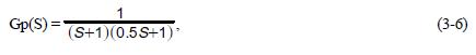
Single-input-single-output:
Gp(S) = Y(S)/U(S) , (3-1)
where, Y(S) is the Laplace transform of y(t), U(S) is the Laplace transform of u(t), and Gp(S) is the open-loop transfer function of the process. - Test Items:
- Linear time-invariant processes with parameter uncertainties.
- Nonlinear in process DC gain.
- Time variant in process time constant.
- Time variant on dead time (or time delay).
- Noisy cases, zero mean noise is added to d(t).
- Structure variation, processes are switched from one to another with different orders and parameters.
- Comparison with PID controller.
- Initial conditions
All the weights are set to small numbers randomly.
r(t) = u(t) = y(t) = 0.
- Input
Step Input r(t) = 1, d(t) = 0, for tracking problem.
r(t) = 0, d(t) = 1, for regulating problem. - Controller Parameters
ANN Response knob is set to 50 percent. It is not adjusted in all the simulations. Sample interval T is set in some cases which will be stated in the simulation.
ANN weights are adjusted automatically.
PID parameters are tuned for certain processes.
- Results
Fig. 2-2 shows the simulation result of a comparison between ANN and PID
control for a second order process with time-constant changes.
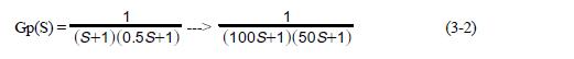
In Fig. 3-2, curve 48 is the step input to the system. Curve 52 shows the system closed-loop step response of ANN control when the dominant time constant (Tc) is 1, and also the identical ANN when Tc is 100.
Curve 54 shows the response of PID control when Tc is 1, and curve 56 shows the response of the PID when Tc is 100.
The sample interval T is a function of Tc but no other parameters of either controller have been changed. It is seen that even if the time constants have changed as large as 100 times, the response of ANN control has no change. On the other hand, the time constant change makes PID control unstable.
Fig. 3-3 shows the simulation result of a comparison between ANN and PID control for a second order plus delay process with dead time changes:
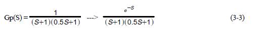
In Fig. 3-3, Curve 60 and 62 show the responses of ANN control when there is no delay and delay is 1, respectively. Curve 64 and 66 show the PID responses in the absence of delay and delay is 1, respectively.
No parameters of either controller have been changed in this instance. It is seen that the ANN controller has a much better control performance than the PID regarding the time delay change.
Fig. 3-4 shows the simulation result of ANN control for a nonlinear process, in which the DC gain varies as a function of r(t):
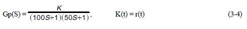
In Fig. 3-4, Curves 74 and 76 show the responses of ANN control when r(t) changes from 0 to 1 (Curve 74), and 1 to 2 (Curve 76), respectively. It is seen that the ANN works well for the process with a nonlinear gain.
Fig. 3-5 shows the simulation result of ANN control for a time-variant process, in which the dominant time constant varies as a function of time:
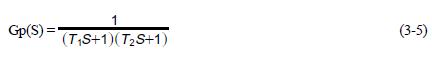
where T1 = 0.25t + 10 , T2 = 0.05t + 5 .
In Fig. 3-5, curve 82 shows the response of ANN control when T1 changes from 10 to 30, and T2 changes from 5 to 10. The sample interval T is selected based on a nominal dominant time constant of 20 and is not changed. It is seen that the ANN works well for controlling time-variant processes.
Fig. 3-6 is the simulation result of ANN control for a system with measurement noise. In this case
where y(t) = y1(t) + d(t), y1(t) is the process output, and d(t) is white noise with zero mean value, and y(t) is the measured variable.
In Fig. 3-6, curve 86 is the step response of ANN control. It is seen that the ANN controller works normally when measurement random noise is applied.